SUPPLEMENTAL DOCUMENT SD-6
FOR PART IVC
– Quality Assurance/Uncertainty
Measurement Uncertainty for Extrapolations of
Net Weight and Unit Count
Table of Contents
Introduction………………………………………………………………………………….…...2
A Example
1: Extrapolation of net weight ………………………………………………3
B Example
2: Extrapolation of net weight in conjunction with a hypergeometric sampling
plan…………………………………………………………….…………….10
C Example
3: Extrapolation of unit count……………………………………………...16
D References……………………………………………………………………………..23
Introduction
The following examples demonstrate various approaches for deriving
estimates of uncertainty associated with weight and count extrapolations:
A Example 1:
Extrapolation of net weight
B Example 2:
Extrapolation of net weight in conjunction with a hypergeometric sampling plan
C Example 3:
Extrapolation of unit count
These examples are meant to be illustrative, not exclusive. Laboratories
should develop defensible procedures that fit their operational environment and
jurisdictional requirements. Notes and calculations are provided to clarify
these applications. Weight calculations are based upon assumptions that
populations are normally distributed.[1]
Various terms used in this document are defined in the SWGDRUG
Recommendations Annex A. The following examples should not be directly applied
to methodology used without first considering the specific purpose of the
method and its relevant operational environment.
A Example 1:
Extrapolation of net weight
Scenario:
A laboratory receives an exhibit containing
100 bags of white powder.
Objective:
The analyst needs to determine the total net
weight of the powder in the 100 bags.
This is done by weighing the powder from a sample of the population and
extrapolating to the total population.[2]
Procedure:
A.1
Determine the population size N.
Only bags which have sufficient similar characteristics are placed in
the same population.
In this
example, the contents of all 100 bags are visually consistent in substance
amount (about 0.5 gram) and physical appearance (i.e. color, texture, etc.),[3]
hence N = 100.
A.2
Select the sample size, n, to be weighed.1
In this
example, the analyst chooses a sample size n
= 10. The 10 units are randomly
selected[4]
from the total population.
(Results for
other n values are given later in the
section.)
A.3
Measure the weight of the powder in each of the
randomly selected units.
The weight (X) of the powder in each of the 10 bags
is measured by dynamic weighing on a three-place balance (with 0.001 gram
readability)[5]
as recorded in table 1.1.
Table 1.1: Individual weights of 10 bags.
|
Bag |
Wt of powder (X), gram |
Bag |
Wt of powder (X), gram |
|
1 |
0.593 |
6 |
0.574 |
|
2 |
0.509 |
7 |
0.580 |
|
3 |
0.557 |
8 |
0.540 |
|
4 |
0.548 |
9 |
0.532 |
|
5 |
0.569 |
10 |
0.529 |
A.4
Calculate the average weight per unit, ![]() , the standard deviation, s, and the relative standard deviation, RSD.
, the standard deviation, s, and the relative standard deviation, RSD.
Average weight per unit, |
= 0.5531 gram |
|
Standard deviation, s |
= 0.02622 gram |
|
Relative Standard Deviation, RSD[6] |
= |
A.5
Obtain the standard uncertainty (unexpanded),
![]() , associated with the balance used.5
, associated with the balance used.5
In this example, the laboratory has determined ![]() = 0.00185 gram for
a three-place balance.
= 0.00185 gram for
a three-place balance.
A.6
Obtain the uncertainty associated with the
calculated average weight, ![]() . This uncertainty
encompasses the standard deviation as well as the number of measurements
performed.
. This uncertainty
encompasses the standard deviation as well as the number of measurements
performed.
![]() = 0.008292
= 0.008292
A.7
Calculate the combined uncertainty, ![]() , associated with the average weight per unit, by
combining the standard uncertainties[7] of the average weight,
, associated with the average weight per unit, by
combining the standard uncertainties[7] of the average weight, ![]() , and the balance used,
, and the balance used, ![]() ,[8] via the
root-sum-square (RSS) method.
,[8] via the
root-sum-square (RSS) method.
![]() = 0.008496 gram
= 0.008496 gram
A.8
Calculate the extrapolated net weight of the
100 bags, W, and its associated
uncertainty, ![]() .
.
Extrapolated
net weight, W = N * ![]() = 100 * 0.5531
g = 55.31 grams
= 100 * 0.5531
g = 55.31 grams
Extrapolated uncertainty, ![]() = N *
= N * ![]() = 100* 0.008496 g = 0.8496 grams
= 100* 0.008496 g = 0.8496 grams
A.9
Obtain the expanded extrapolated uncertainty,
![]() , by using the appropriate coverage factor, k, (Student’s t value for 9 degrees of freedom).[9] Round up the expanded extrapolated uncertainty,
, by using the appropriate coverage factor, k, (Student’s t value for 9 degrees of freedom).[9] Round up the expanded extrapolated uncertainty,
![]() , to two significant figures.[10]
, to two significant figures.[10]
If a 95% level of confidence is used, (coverage factor k = 2.262),
![]() =
= ![]() * k = 0.8496 g * 2.262 = 1.921 grams » 2.0 grams
* k = 0.8496 g * 2.262 = 1.921 grams » 2.0 grams
If a 99% level of confidence is used (coverage factor k = 3.250),
![]() =
= ![]() * k = 0.8496 g * 3.250 = 2.761 grams » 2.8 grams
* k = 0.8496 g * 3.250 = 2.761 grams » 2.8 grams
A.10 Report the total extrapolated net weight and its
associated uncertainty by truncating the extrapolated net weight to the same
level of significance (i.e. decimal places) as the rounded expanded uncertainty.
When the 95% level of confidence is used:
The amount of powder in 100 bags is 55.3 grams ± 2.0 grams at a 95% level of confidence, determined by
weighing 10 bags and extrapolating to obtain the total net weight.
When the 99% level of confidence is used:
The amount of powder in 100 bags is 55.3 grams ± 2.8
grams at a 99% level of confidence, determined by weighing 10 bags and
extrapolating to obtain the total net weight.
A.11 If the
analyst also performs qualitative analysis on each one of the 10 randomly
selected bags and all are found to contain cocaine (that is, no negatives
found), the following inferences about the population (at the respective 95% or
99% levels of confidence) can be made:
By statistically
sampling 10 bags, it is concluded at a 95% level of confidence, that at least
76% of the population contains cocaine.
By statistically
sampling 10 bags, it is concluded at a 99% level of confidence, that at least
65% of the population contains cocaine.
The above
statistical inferences on the population as well as for other levels of
confidence (depending on laboratory’s policy and decision), can be calculated
using the ENFSI DWG Calculator for Qualitative Sampling of Seized Drugs (Reference
D.2). This calculator can also be accessed from the SWGDRUG website at http://www.swgdrug.org/tools.htm).
Appendix 1.1:
Net weights and associated uncertainties
extrapolated for other sample sizes are given in Table 1.2. It is noted that as the sample size n increases, the expanded extrapolated
uncertainty, ![]() , decreases. Also,
for a given sample size n, the
expanded uncertainty is larger when a higher level of confidence is used.
, decreases. Also,
for a given sample size n, the
expanded uncertainty is larger when a higher level of confidence is used.
Table 1.2: Calculations
for sample sizes of n = 3, 5, 10, 20
and 30.
|
Sample size, n |
3 |
5 |
10 |
20 |
30 |
|
Avg wt of unit, |
0.5530 |
0.5552 |
0.5531 |
0.5514 |
0.5510 |
|
Std deviation, s |
0.04214 |
0.03086 |
0.02622 |
0.02860 |
0.02759 |
|
% RSD |
7.621 |
5.558 |
4.741 |
5.188 |
5.007 |
|
Std uncertainty of avg wt, |
0.024331 |
0.013800 |
0.008292 |
0.006396 |
0.005037 |
|
Combined std uncertainty, |
0.024401 |
0.013923 |
0.008496 |
0.006658 |
0.005366 |
|
Extrapolated uncertainty, |
2.4401 |
1.3923 |
0.8496 |
0.6658 |
0.5366 |
|
Extrapolated wt, W |
55.30 |
55.52 |
55.31 |
55.14 |
55.10 |
|
With 95% Level of
Confidence |
|||||
|
Coverage factor, k |
4.303 |
2.776 |
2.262 |
2.093 |
2.045 |
|
Exp extrapolated uncertainty, |
10.499 |
3.865 |
1.922 |
1.394 |
1.097 |
|
Lower Wt Limit |
44.80 |
51.65 |
53.39 |
53.74 |
54.00 |
|
Upper Wt Limit |
65.80 |
59.39 |
57.23 |
56.53 |
56.20 |
|
With 99% Level of
Confidence |
|||||
|
Coverage factor, k |
9.925 |
4.604 |
3.250 |
2.861 |
2.756 |
|
Exp extrapolated
uncertainty, |
24.218 |
6.410 |
2.761 |
1.905 |
1.479 |
|
Lower Wt Limit |
31.08 |
49.11 |
52.55 |
53.23 |
53.62 |
|
Upper Wt Limit |
79.52 |
61.93 |
58.07 |
57.04 |
56.58 |
Raw data of individual sample weights used
are given in Table 1.3.
Table 1.3:
Individual sample weights of 30 bags used in examples.
|
Bag |
Wt of powder (X),
gram |
Bag |
Wt of powder (X),
gram |
Bag |
Wt of powder (X),
gram |
|
1 |
0.593 |
11 |
0.583 |
21 |
0.593 |
|
2 |
0.509 |
12 |
0.510 |
22 |
0.530 |
|
3 |
0.557 |
13 |
0.540 |
23 |
0.548 |
|
4 |
0.548 |
14 |
0.582 |
24 |
0.581 |
|
5 |
0.569 |
15 |
0.552 |
25 |
0.539 |
|
6 |
0.574 |
16 |
0.530 |
26 |
0.579 |
|
7 |
0.580 |
17 |
0.509 |
27 |
0.530 |
|
8 |
0.540 |
18 |
0.580 |
28 |
0.532 |
|
9 |
0.532 |
19 |
0.520 |
29 |
0.511 |
|
10 |
0.529 |
20 |
0.590 |
30 |
0.560 |
Step A.7 shows that the combined uncertainty,![]() , has contributions from: the standard uncertainties of
the average weight,
, has contributions from: the standard uncertainties of
the average weight, ![]() , and that associated with the balance used,
, and that associated with the balance used, ![]() . If a balance of
a different uncertainty is used, the combined uncertainty will change. Similarly, the distribution of the individual
weights of the population will affect the combined uncertainty. To illustrate the impact of the weight
distribution of the population on the extrapolation of the total net weight,
another 30 bags from a different population (one that has been tested to be
normally distributed) are individually weighed on the same balance. The individual weights of these 30 bags are
given in Table 1.4 below and the associated calculations given in Table
1.5. It is noted that the RSD values
listed in Table 1.5 are all much smaller than those for Table 1.2 (above). This consequentially gives rise to smaller
expanded extrapolated uncertainty,
. If a balance of
a different uncertainty is used, the combined uncertainty will change. Similarly, the distribution of the individual
weights of the population will affect the combined uncertainty. To illustrate the impact of the weight
distribution of the population on the extrapolation of the total net weight,
another 30 bags from a different population (one that has been tested to be
normally distributed) are individually weighed on the same balance. The individual weights of these 30 bags are
given in Table 1.4 below and the associated calculations given in Table
1.5. It is noted that the RSD values
listed in Table 1.5 are all much smaller than those for Table 1.2 (above). This consequentially gives rise to smaller
expanded extrapolated uncertainty,![]() , for all sample sizes in Table 1.5 as compared to Table
1.2.
, for all sample sizes in Table 1.5 as compared to Table
1.2.
Table 1.4:
Individual sample weights of 30 bags from a normally distribution population.
|
Bag |
Wt of powder (X),
gram |
Bag |
Wt of powder (X),
gram |
Bag |
Wt of powder (X),
gram |
|
1 |
0.553 |
11 |
0.557 |
21 |
0.552 |
|
2 |
0.549 |
12 |
0.557 |
22 |
0.554 |
|
3 |
0.557 |
13 |
0.552 |
23 |
0.555 |
|
4 |
0.554 |
14 |
0.555 |
24 |
0.557 |
|
5 |
0.550 |
15 |
0.555 |
25 |
0.551 |
|
6 |
0.553 |
16 |
0.556 |
26 |
0.557 |
|
7 |
0.556 |
17 |
0.557 |
27 |
0.557 |
|
8 |
0.557 |
18 |
0.547 |
28 |
0.556 |
|
9 |
0.555 |
19 |
0.554 |
29 |
0.551 |
|
10 |
0.556 |
20 |
0.556 |
30 |
0.552 |
Table 1.5: Calculations
for sample sizes of n = 3, 5, 10, 20
and 30.
|
Sample
size, n |
3 |
5 |
10 |
20 |
30 |
|||
|
Avg wt of unit, |
0.5530 |
0.5526 |
0.5540 |
0.5543 |
0.5543 |
|||
|
Std deviation, s |
0.004000 |
0.003209 |
0.002789 |
0.002886 |
0.002728 |
|||
|
% RSD |
0.7233 |
0.5808 |
0.5034 |
0.5206 |
0.4922 |
|||
|
Std uncertainty of avg wt, |
0.0023094 |
0.0014353 |
0.0008819 |
0.0006452 |
0.0004981 |
|||
|
Combined std uncertainty, |
0.002959 |
0.002341 |
0.002049 |
0.001959 |
0.001916 |
|||
|
Extrapolated uncertainty, |
0.2959 |
0.2341 |
0.2049 |
0.1959 |
0.1916 |
|||
|
Extrapolated wt, W |
55.30 |
55.26 |
55.40 |
55.43 |
55.43 |
|||
|
With 95% Level of
Confidence |
||||||||
|
Coverage factor, k |
4.303 |
2.776 |
2.262 |
2.093 |
2.045 |
|||
|
Exp extrapolated
uncertainty, |
1.273 |
0.650 |
0.463 |
0.410 |
0.392 |
|||
|
Lower Wt Limit |
54.03 |
54.61 |
54.94 |
55.02 |
55.04 |
|||
|
Upper Wt Limit |
56.57 |
55.91 |
55.86 |
55.84 |
55.82 |
|||
|
With 99% Level of
Confidence |
||||||||
|
Coverage factor, k |
9.925 |
4.604 |
3.250 |
2.860 |
2.756 |
|||
|
Exp extrapolated uncertainty, |
2.937 |
1.078 |
0.666 |
0.560 |
0.528 |
|||
|
Lower Wt Limit |
52.36 |
54.18 |
54.73 |
54.87 |
54.90 |
|||
|
Upper Wt Limit |
58.24 |
56.34 |
56.07 |
55.99 |
55.95 |
|||
B Example
2: Extrapolation of net weight in conjunction
with a hypergeometric sampling plan
Scenario:
The scenario is the same as Example 1, where
the laboratory receives an exhibit
containing 100 bags of white powder.
Sentencing penalty in this jurisdiction increases if the amount of
substance containing cocaine exceeds 25 grams.
Objective:
The analyst
will use statistically based sampling without replacement to determine, to a
99% level of confidence, if the jurisdictional weight threshold is exceeded. This
example does not take purity of the powder into account because it is not
jurisdictionally relevant.
Procedure:
B.1
The analyst needs to determine how many bags must
be sampled to determine if the 25-gram threshold weight is exceeded.
To obtain an estimation of the number of bags that must be
sampled to meet the threshold weight, the specified statutory threshold weight
(25 grams) is divided by the average net weight (![]() ) per unit (obtained from Example 1).
) per unit (obtained from Example 1).
Estimated
number of bags = ![]() = 45.1 (46 bags)
= 45.1 (46 bags)
The extrapolated net weight of 46 bags results in 25.4
grams ± 1.3 grams (See blue dotted line in figure below. The calculation
to estimate the uncertainty of the measurement is not shown here. Refer to Steps B.3 to B.5 below for
calculation process). The lower bound of
24.1 grams falls below the statutory threshold.

To calculate the number of bags needed for the lower
bound of the extrapolated net weight to exceed the statutory threshold weight,
the specified statutory threshold weight (25 grams) is divided by the difference
between the average net weight (![]() ) per unit and the confidence interval with
coverage factor k = 3.250 using Student’s
t value for 9 degrees of freedom based on a sample of 10 bags (see Example
1).
) per unit and the confidence interval with
coverage factor k = 3.250 using Student’s
t value for 9 degrees of freedom based on a sample of 10 bags (see Example
1).
Estimated
number of bags = ![]()
![]() = 47.5 (48 bags)
= 47.5 (48 bags)
Therefore, a minimum of 48 bags must be sampled to
provide strong evidence that the threshold weight is exceeded. The measurement of uncertainty associated
with weighing 48 bags is 1.4 grams at a 99% level of confidence (see detail
calculation in Step B.4), hence giving a lower bound of 25.1 grams, which is
above the statutory threshold. This is
depicted by the green dotted line in the figure above.
B.2
Determine
the sample size n that needs to be
qualitatively tested to demonstrate that at least 48 of the 100 bags contain
cocaine at a 99% level of confidence.
Method 1: 99% level of confidence corresponds
to an a of 0.01 (level of confidence = 0.99 = 1-a). Proceed to use
a hypergeometric sampling calculator to determine the sample size needed. (See Reference D.2)
Using the hypergeometric sampling calculator
and the appropriate parameters
(N =
100, a = 0.01, proportion of positives = 0.48, with
no negatives expected), the sample size is determined to be 6.
or
Method 2: Manually determine the number of
bags, n, to be tested using the established
significance level of 0.01 (corresponding to a 99% level of confidence). In
this instance, there are two possible outcomes or hypotheses:
H1 - Hypothesis that ≥ 48 bags contain cocaine
H0 - Hypothesis that < 48 bags contain cocaine (null hypothesis)
Since the first chance of failure will occur when 47 out of the 100
bags contain cocaine, we want to obtain enough evidence to reject the
assumption that there are only 47 bags of cocaine (H0). This is done by calculating the probability of
obtaining a positive result at successive sample sizes, n, until it falls below the established significance level (a = 0.01).
![]()
![]()
= P (all n bags in the sample contain
cocaine)
The following calculations show the p-values (and resulting levels of
confidence, LoC) obtained for each successive sample tested (with no negatives
found) until a value below 0.01 is obtained (which is sample 6):
![]() 0.4700 (53.00% LoC)
0.4700 (53.00% LoC)
![]() 0.2183 (78.16% LoC)
0.2183 (78.16% LoC)
![]()
![]() 0.1003 (89.97% LoC)
0.1003 (89.97% LoC)
![]() 0.0454 (95.45% LoC)
0.0454 (95.45% LoC)
![]() 0.0203 (97.96% LoC)
0.0203 (97.96% LoC)
![]() 0.0090 (99.10% LoC)
0.0090 (99.10% LoC)
The
probability of randomly selecting 6 units and having them all test positive is
too low to occur by chance (below established significance level) if we assume there
are only 47 positives in the population. Therefore, we can reject H0
and accept H1, that there are ≥ 48 bags that contain cocaine
in the population.
Therefore, the number of bags, n, needed for testing is 6.
B.3
A total of 6 bags are randomly selected for chemical
analysis[11]
and confirmed to contain cocaine. Since
all 6 bags are found to contain cocaine, it can be stated, to a 99% level of
confidence, that at least 48 of the 100 bags contain cocaine.
The
total net weight of 48 bags, W48, can be extrapolated from the
average net weight per unit (obtained from Example 1):
W48 =
48 * ![]() = 48 * 0.5531 g = 26.5488 grams
= 48 * 0.5531 g = 26.5488 grams
B.4
The combined standard
uncertainty, ![]() , associated with the average weight per unit
as calculated from Example 1 is:
, associated with the average weight per unit
as calculated from Example 1 is:
![]() =
0.008496 gram
=
0.008496 gram
The
extrapolated uncertainty for 48 bags, ![]() ,
is calculated as
,
is calculated as
![]() =
0.008496 g * 48 = 0.4078
gram
=
0.008496 g * 48 = 0.4078
gram
The
total expanded uncertainty (![]() ),
at 99% level of confidence, and rounded up to two significant figures (coverage
factor k = 3.250
using Student’s t value for 9 degrees
of freedom since the contents of 10 bags were individually weighed in Step A.2)
is
),
at 99% level of confidence, and rounded up to two significant figures (coverage
factor k = 3.250
using Student’s t value for 9 degrees
of freedom since the contents of 10 bags were individually weighed in Step A.2)
is
![]() =
0.4078 g * 3.250
= 1.3254 g » 1.4 gram
=
0.4078 g * 3.250
= 1.3254 g » 1.4 gram
B.5
The analyst compares the
calculated extrapolated weight of the 48 bags, W48, minus the expanded uncertainty, ![]() , (truncated to the same level of significance) against
the statutory threshold of 25 grams.
, (truncated to the same level of significance) against
the statutory threshold of 25 grams.
The
weight of 48 bags is 26.5 grams ± 1.4 grams calculated at a 99% level of confidence. The lower end of the weight
range is = 26.5 – 1.4 grams =
25.1 grams (which is above 25-grams statutory threshold).
B.6
The results
of the analysis can be reported in either of the following ways:
1) A total of 100 indistinguishable bags were received. By using statistical sampling of 6 bags, it
is concluded at a 99% level of confidence that at least 48% of the population
contains cocaine. The extrapolated net weight of 48 bags is 26.5 grams ± 1.4 grams at a
99% level of confidence.
2) A total of 100 indistinguishable bags were
received. Using statistical (hypergeometric) sampling and by testing 6 bags, it
is concluded that cocaine is present in at least 25.1 grams of powder at a
level of confidence of at least 98%.
Explanation on deriving the overall level of
confidence (i.e. at least 98%):
The second report option gives an overall
level of confidence of at least 98% for the weight and identity of the
powder. Each of these parameters is
individually tested at a 99% level of confidence. Where these two statements are not considered
to be independent of each other, the Bonferroni correction (Reference D.1, p
155-156) can be used in the calculation of the overall confidence level. This is obtained by determining the value of
(1 – 0.01 – 0.01)*100%. If the two
statements are considered independent, the multiplication rule of probability
can be used instead, giving an overall level of confidence of 99%*99% =
98.01%.
Appendix 2.1:
To contrast the practicality of using
hypergeometric sampling to identify a proportion of a population, the following
example is given:
If a
sampling size of 6 is used to determine the content of all 100 bags, the
probability of failure (finding less than 100 bags containing cocaine) = ![]()
![]()
![]()
As
illustrated in this case, if only 6 bags are sampled, the analyst is only 6%
confident that all 100 bags contain a substance containing cocaine.
If a 95% level of confidence is needed for the reporting
of content of all 100 bags, the sampling size needs to be increased as shown
below:
![]()
giving a sample size of 95.
Therefore,
it is often practical to report that a certain proportion of the population is
positive instead of reporting on the entire population. This can be achieved by using statistical
sampling. Using the same example of a total population of 100 bags, if the
laboratory only needs to report on the content of 90 bags, the sampling size
would reduce to 23:
![]()
As seen
from this example, if the laboratory needs to report on the content of all 100
bags at a confidence level of 95%, a total of 95 bags need to be tested. In contrast, if the laboratory only needs to
report on the content of 90 bags at the same confidence level, the number of
bags to be tested is reduced to 23 (a reduction of 75%).
C Example
3: Extrapolation of unit count
Scenario:
The laboratory receives a large container
with numerous tablets.
Objective:
The analyst needs to determine the total
number of tablets present in the container and its associated uncertainty by
direct weighing of a sample of individual tablets and extrapolating to obtain
the total count.
Procedure:
C.1
Determine whether all the tablets in the
container can be treated as one population.
Since all the tablets in the container are visually
similar, they will be treated as one population.
C.2
Measure the net weight of all the tablets.
The total weight, TW,
of the total population of tablets is determined to be 701.5 grams based on
dynamic weighing on a balance with 0.1 gram readability.
C.3
Choose the number of individual tablets to
weigh.
In this example, the analyst randomly samples and weighs
10 tablets (n = 10).
(Results for other n
values are given later in the section.)
The weight of each tablet X is determined by dynamic weighing on a balance with 0.0001 gram
readability as in Table 3.1.
Table 3.1: Individual weights of 10 tablets.
|
Tablet |
Wt of tablet (X), gram |
Tablet |
Wt of tablet (X), gram |
|
1 |
0.3084 |
6 |
0.3437 |
|
2 |
0.3225 |
7 |
0.2918 |
|
3 |
0.3349 |
8 |
0.3116 |
|
4 |
0.2981 |
9 |
0.3077 |
|
5 |
0.3293 |
10 |
0.3426 |
C.4
Calculate the average weight per tablet, ![]() , the standard
deviation of the tablet weight, s,
and the relative standard deviation, RSD.
, the standard
deviation of the tablet weight, s,
and the relative standard deviation, RSD.
|
Average weight per tablet, |
= 0.31906 gram |
|
Standard deviation, s |
= 0.018287 gram |
|
Relative standard deviation, RSD |
= 5.7314 % |
C.5
The number of tablets in the container is
estimated by dividing the total weight of all the tablets, TW, by the average weight per tablet, ![]() .
.
Estimated
number of tablets in container = ![]() 2198.6
2198.6
C.6
Obtain the uncertainty associated with the
two balances used5:
Uncertainty for one-place balance (0.1 g readability), ![]() = 0.35810 gram
= 0.35810 gram
Uncertainty
for four-place balance (0.0001 g readability), ![]() = 0.0004840 gram
= 0.0004840 gram
C.7
Calculate the relative uncertainties of both
weighing processes. The use of relative
standard uncertainties is necessary because the estimated number of tablets is
obtained by a division operation (see C.5).
Relative
uncertainty of the total weight of tablets, ![]() :
:
![]() 0.00051048
0.00051048
Relative uncertainty of average weight per tablet, ![]() :
:
 = 0.018188
C.8
Combine the two relative standard
uncertainties (![]() and
and ![]() ) to obtain the combined relative standard uncertainty,
) to obtain the combined relative standard uncertainty,![]() , associated with the extrapolated tablet count.
, associated with the extrapolated tablet count.
![]() =
0.018195
=
0.018195
C.9
Determine the absolute combined uncertainty, ![]() , for the tablet count by multiplying the combined
relative standard uncertainty,
, for the tablet count by multiplying the combined
relative standard uncertainty, ![]() , by the estimated
number of tablets.
, by the estimated
number of tablets.
![]() number of tablets= 0.018195 * 2198.6 = 40.004
number of tablets= 0.018195 * 2198.6 = 40.004
C.10
Expand the combined uncertainty, ![]() , using the appropriate coverage factor k.
, using the appropriate coverage factor k.
At a 95% level of confidence for n = 10, the coverage factor k
= 2.262.
Expanded
uncertainty, ![]() =
= ![]() * k = 40.004 * 2.262 = 90.489 tablets.
* k = 40.004 * 2.262 = 90.489 tablets.
If a 99% level of confidence is used, the coverage factor
k = 3.250.
Expanded
uncertainty, ![]() =
= ![]() * k = 40.004 * 3.250 = 130.013 tablets.
* k = 40.004 * 3.250 = 130.013 tablets.
C.11
Report the total extrapolated tablet number,
and its associated uncertainty, truncating or rounding to the nearest whole
number per laboratory policy. In this
example, the number of tablets is truncated while the associated uncertainty is
rounded up for a conservative approach.
Number of tablets: 2198 ± 91
The number of tablets is an
extrapolated estimated value based on the individual weights of 10 tablets and
the uncertainty value represents an expanded uncertainty at a 95% level of
confidence.
Number of tablets: 2198 ± 131
The number of tablets is an
extrapolated estimated value based on the individual weights of 10 tablets and
the uncertainty value represents an expanded uncertainty at a 99% level of
confidence.
Appendix 3.1:
Examples of other sample sizes n = 3, 5, 30 and 50 taken from the same
population are given in Table 3.2, together with data from n = 10 for comparison. Raw
data of tablet weights used for Table 3.2 are given in Table 3.3. It is noted
that the extrapolated combined uncertainty, ![]() , is smaller as the sample size gets bigger. Also, for a given sample size n, the expanded uncertainty,
, is smaller as the sample size gets bigger. Also, for a given sample size n, the expanded uncertainty, ![]() , is larger when a higher level of confidence is used.
, is larger when a higher level of confidence is used.
It should be the laboratory’s decision and
policy to determine the sample size n
needed for the extrapolation of number of units. Using a smaller n is more time efficient but results in a much larger expanded
uncertainty, ![]() . Using a larger n takes more time to complete the
analysis but has the benefit of a smaller expanded uncertainty.
. Using a larger n takes more time to complete the
analysis but has the benefit of a smaller expanded uncertainty.
Table 3.2: Calculations
for sample sizes of n =3, 5, 10, 30
and 50.
|
Sample size, n |
3 |
5 |
10 |
30 |
50 |
|
Avg wt per tablet, |
0.32193 |
0.31864 |
0.31906 |
0.32337 |
0.32510 |
|
Std deviation, s |
0.013259 |
0.015163 |
0.018287 |
0.017731 |
0.019186 |
|
% RSD |
4.1186 |
4.7587 |
5.7314 |
5.4833 |
5.9016 |
|
Extrapolated tablet count, |
2179.0 |
2201.5 |
2198.6 |
2169.3 |
2157.8 |
|
Std uncertainty of avg wt, |
0.0076551 |
0.0067811 |
0.0057828 |
0.0032373 |
0.0027133 |
|
Rel. uncertainty of net wt, |
0.00051048 |
0.00051048 |
0.00051048 |
0.00051048 |
0.00051048 |
|
Rel. uncertainty of avg wt, |
0.023826 |
0.021336 |
0.018188 |
0.010122 |
0.008478 |
|
Combined relative uncertainty, |
0.023832 |
0.021342 |
0.018195 |
0.010135 |
0.008493 |
|
Extrapolated combined uncertainty, |
51.930 |
46.985 |
40.004 |
21.987 |
18.327 |
|
With 95% Level of
Confidence |
|||||
|
Coverage factor, k |
4.302 |
2.776 |
2.262 |
2.045 |
2.010 |
|
Expanded uncertainty, |
223.403 |
130.430 |
90.489 |
44.963 |
36.837 |
|
With 99% Level of
Confidence |
|||||
|
Coverage factor, k |
9.924 |
4.604 |
3.250 |
2.756 |
2.680 |
|
Expanded uncertainty, |
515.353 |
216.319 |
130.013 |
60.596 |
49.116 |
Table 3.3:
Individual weight of tablets for Table 3.2.
|
Tablet |
Wt of tablet (X), gram |
Tablet |
Wt of tablet (X), gram |
Tablet |
Wt of tablet (X), gram |
|
1 |
0.3084 |
21 |
0.3152 |
41 |
0.3580 |
|
2 |
0.3225 |
22 |
0.2763 |
42 |
0.3090 |
|
3 |
0.3349 |
23 |
0.3058 |
43 |
0.3251 |
|
4 |
0.2981 |
24 |
0.3014 |
44 |
0.3459 |
|
5 |
0.3293 |
25 |
0.3376 |
45 |
0.3054 |
|
6 |
0.3437 |
26 |
0.3313 |
46 |
0.3195 |
|
7 |
0.2918 |
27 |
0.3388 |
47 |
0.2802 |
|
8 |
0.3116 |
28 |
0.3192 |
48 |
0.3463 |
|
9 |
0.3077 |
29 |
0.3323 |
49 |
0.2802 |
|
10 |
0.3426 |
30 |
0.3348 |
50 |
0.3356 |
|
11 |
0.3476 |
31 |
0.3462 |
|
|
|
12 |
0.3450 |
32 |
0.3317 |
|
|
|
13 |
0.3196 |
33 |
0.3322 |
|
|
|
14 |
0.3171 |
34 |
0.3272 |
|
|
|
15 |
0.3321 |
35 |
0.3305 |
|
|
|
16 |
0.3441 |
36 |
0.3383 |
|
|
|
17 |
0.3435 |
37 |
0.3456 |
|
|
|
18 |
0.3240 |
38 |
0.3456 |
|
|
|
19 |
0.3293 |
39 |
0.3106 |
|
|
|
20 |
0.3155 |
40 |
0.3408 |
|
|
Appendix 3.2:
To illustrate the impact of the weight
distribution on the extrapolation of the unit count, three distinct populations
of weights of tablets were evaluated.
All groups contain 50 tablets.
Tablets from each group look visually
similar. The total weight of each group
of 50 tablets is weighed using a one-place balance (with uncertainty of 0.3581
gram). A sample size of 10 tablets from
each group is randomly sampled for individual weighing using a four-place
balance (with uncertainty of 0.000484 gram).
The calculations for the extrapolation of tablet count for the three
groups are shown in Table 3.4 below.
The RSD of the sample, and hence the expanded
uncertainty of the extrapolation, depends on the distribution curve. A population with a smaller spread will yield
a smaller standard deviation and hence smaller expanded uncertainty.
Table 3.4:
Calculations for 3 groups of tablets each with sample sizes of 10.
|
|
Group 1 |
Group 2 |
Group 3 |
|
Total Weight of 50 tablets, TW, gram |
16.3 |
28.7 |
27.9 |
|
Avg weight per tablet, |
0.31906 |
0.58253 |
0.55591 |
|
Std deviation, s |
0.018287 |
0.011608 |
0.0052800 |
|
% RSD |
5.73142 |
1.9926 |
0.94980 |
|
Extrapolated tablet count, |
51.088 |
49.268 |
50.188 |
|
Std uncertainty of avg wt, |
0.0181877 |
0.0036706 |
0.0016697 |
|
Rel. uncertainty of total wt, |
0.021969 |
0.012477 |
0.012835 |
|
Rel. uncertainty of avg wt, |
0.0181877 |
0.0063557 |
0.0031272 |
|
Combined rel uncertainty, |
0.028521 |
0.014003 |
0.013211 |
|
Extrapolated combined uncertainty, |
1.45707 |
0.68989 |
0.66301 |
|
With Level of Confidence
= 95% (k = 2.262) |
|||
|
Expanded uncertainty, |
3.296 |
1.561 |
1.500 |
|
With Level of Confidence
= 99% (k = 3.250) |
|||
|
Expanded uncertainty, |
4.735 |
2.242 |
2.155 |
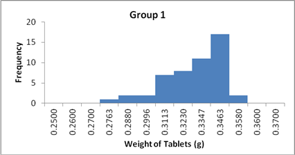
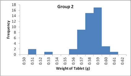
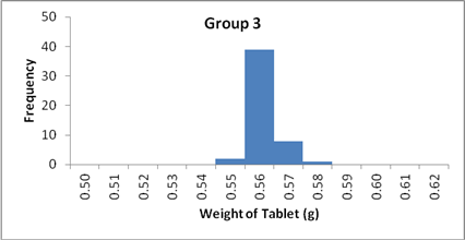
Figure 1: Histograms showing the spread of weights for the 50 tablets in
the three groups. The spread of the data
in group 1 is larger and further from normality as compared to Group 3.
D References
D.1
Kutner, M. H., Nachtsheim,
C. J., and Neter, J. 2004. Applied Linear Regression Models, 4th edition,
McGraw-Hill.
D.2
ENFSI-DWG Guidelines on Sampling of Illicit Drugs
for Qualitative Analysis (2016). http://enfsi.eu/wp-content/uploads/2017/05/guidelines_on_sampling_of_illicit_drugs_for_qualitative_analysis_enfsi_dwg_2nd_edition.pdf
D.3
EURACHEM/CITAC Guide. Quantifying Uncertainty
in Analytical Measurement, Third Edition (2012). ISBN 978-0-948926-30-3.
D.4
Guide to the Expression of Uncertainty in
Measurement (GUM). ISO, Geneva (1993). (ISBN 92-67-10188-9) (Reprinted 1995:
Reissued as ISO Guide 98-3 (2008), also available from http://www.bipm.org as
JCGM 100:2008).
D.5
ASCLD/LAB. 2013. ASCLD/LAB Policy on Measurement
Uncertainty. AL-PD-3060 Ver 1.0.
D.6
Mario, J. 2010. A probability-based sampling
approach for the analysis of drug seizures composed of multiple containers of
either cocaine, heroin, or Cannabis. Forensic
Science International 197: 105-113.